Moisture Advection

import numpy as np
import matplotlib.pyplot as plt
import metpy.calc as mcalc 
from metpy.units import units
import glob
import xarray as xr

from datetime import datetime, timedelta
from functools import partial
import numpy as np
import pandas as pd
import xarray as xr

import matplotlib
import matplotlib.animation as animation
import matplotlib.pyplot as plt
import matplotlib.gridspec as gridspec
from matplotlib.colors import Normalize

path_staging = "/data/project/ARM_Summer_School_2024_Data/lasso_tutorial/cacti/lasso-cacti"
file_list = sorted(glob.glob(f'{path_staging}/20190129/eda09/base/les/subset_d3/corlasso_met_*'))

ds = xr.open_dataset(file_list[30])

ds

<xarray.Dataset> Size: 6GB
Dimensions:               (Time: 1, south_north: 865, west_east: 750,
                           bottom_top: 149)
Coordinates:
  * Time                  (Time) datetime64[ns] 8B 2019-01-29T13:30:00
    XLONG                 (south_north, west_east) float32 3MB ...
    XLAT                  (south_north, west_east) float32 3MB ...
    XTIME                 (Time) float32 4B ...
Dimensions without coordinates: south_north, west_east, bottom_top
Data variables: (12/52)
    ITIMESTEP             (Time) int32 4B ...
    MUTOT                 (Time, south_north, west_east) float32 3MB ...
    HGT                   (Time, south_north, west_east) float32 3MB ...
    HAMSL                 (Time, bottom_top, south_north, west_east) float32 387MB ...
    P_HYD                 (Time, bottom_top, south_north, west_east) float32 387MB ...
    PRESSURE              (Time, bottom_top, south_north, west_east) float32 387MB ...
    ...                    ...
    MULFC                 (Time, south_north, west_east) float32 3MB ...
    MULNB                 (Time, south_north, west_east) float32 3MB ...
    MULPL                 (Time, south_north, west_east) float32 3MB ...
    MUCAPE                (Time, south_north, west_east) float32 3MB ...
    MUCIN                 (Time, south_north, west_east) float32 3MB ...
    REFL_10CM_MAX         (Time, south_north, west_east) float32 3MB ...
Attributes: (12/39)
    DX:                          500.0
    DY:                          500.0
    SIMULATION_START_DATE:       2019-01-29_06:00:00
    WEST-EAST_GRID_DIMENSION:    751
    SOUTH-NORTH_GRID_DIMENSION:  866
    BOTTOM-TOP_GRID_DIMENSION:   150
    ...                          ...
    doi_isPartOf_lasso-cacti:    https://doi.org/10.5439/1905789
    doi_isDocumentedBy:          https://doi.org/10.2172/1905845
    doi_thisFileType:            https://doi.org/10.5439/1905819
    history:                     processed by user d3m088 on machine cirrus89...
    filename_user:               corlasso_met_2019012900eda09d3_base_M1.m1.20...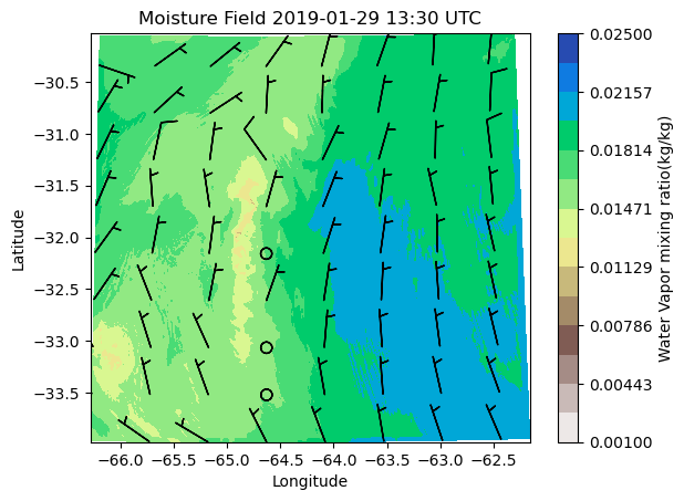
    filename_storage:            corlassomet2019012900eda09d3baseM1.m1.201901...

xarray.Dataset

• Dimensions:
  • Time: 1
  • south_north: 865
  • west_east: 750
  • bottom_top: 149
• Coordinates: (4)
  • Time
    (Time)
    datetime64[ns]
    2019-01-29T13:30:00

    array(['2019-01-29T13:30:00.000000000'], dtype='datetime64[ns]')

  • XLONG
    (south_north, west_east)
    float32
    ...

    [648750 values with dtype=float32]

  • XLAT
    (south_north, west_east)
    float32
    ...

    [648750 values with dtype=float32]

  • XTIME
    (Time)
    float32
    ...

    [1 values with dtype=float32]

• Data variables: (52)
  • ITIMESTEP
    (Time)
    int32
    ...

    description :

    WRF timestep number since run start

    units :

    [1 values with dtype=int32]

  • MUTOT
    (Time, south_north, west_east)
    float32
    ...

    description :

    dry air mass in column

    units :

    Pa

    stagger :

    [648750 values with dtype=float32]

  • HGT
    (Time, south_north, west_east)
    float32
    ...

    description :

    Terrain Height

    units :

    m

    stagger :

    [648750 values with dtype=float32]

  • HAMSL
    (Time, bottom_top, south_north, west_east)
    float32
    ...

    description :

    model height - [MSL] (mass grid)

    units :

    m

    stagger :

    [96663750 values with dtype=float32]

  • P_HYD
    (Time, bottom_top, south_north, west_east)
    float32
    ...

    description :

    hydrostatic pressure

    units :

    Pa

    stagger :

    [96663750 values with dtype=float32]

  • PRESSURE
    (Time, bottom_top, south_north, west_east)
    float32
    ...

    description :

    pressure

    units :

    hPa

    stagger :

    [96663750 values with dtype=float32]

  • ALT
    (Time, bottom_top, south_north, west_east)
    float32
    ...

    description :

    inverse density

    units :

    m3 kg-1

    stagger :

    [96663750 values with dtype=float32]

  • TEMPERATURE
    (Time, bottom_top, south_north, west_east)
    float32
    ...

    description :

    temperature

    units :

    K

    stagger :

    [96663750 values with dtype=float32]

  • THETA
    (Time, bottom_top, south_north, west_east)
    float32
    ...

    description :

    potential temperature

    units :

    K

    stagger :

    [96663750 values with dtype=float32]

  • THETA_E
    (Time, bottom_top, south_north, west_east)
    float32
    ...

    description :

    equivalent potential temperature

    units :

    K

    stagger :

    [96663750 values with dtype=float32]

  • QVAPOR
    (Time, bottom_top, south_north, west_east)
    float32
    ...

    description :

    Water vapor mixing ratio

    units :

    kg kg-1

    stagger :

    [96663750 values with dtype=float32]

  • RH
    (Time, bottom_top, south_north, west_east)
    float32
    ...

    description :

    relative humidity

    units :

    %

    stagger :

    [96663750 values with dtype=float32]

  • UA
    (Time, bottom_top, south_north, west_east)
    float32
    ...

    description :

    destaggered u-wind component

    units :

    m s-1

    stagger :

    [96663750 values with dtype=float32]

  • VA
    (Time, bottom_top, south_north, west_east)
    float32
    ...

    description :

    destaggered v-wind component

    units :

    m s-1

    stagger :

    [96663750 values with dtype=float32]

  • WA
    (Time, bottom_top, south_north, west_east)
    float32
    ...

    description :

    destaggered w-wind component

    units :

    m s-1

    stagger :

    [96663750 values with dtype=float32]

  • UMET
    (Time, bottom_top, south_north, west_east)
    float32
    ...

    description :

    earth-relative u-wind component

    units :

    m s-1

    stagger :

    [96663750 values with dtype=float32]

  • VMET
    (Time, bottom_top, south_north, west_east)
    float32
    ...

    description :

    earth-relative v-wind component

    units :

    m s-1

    stagger :

    [96663750 values with dtype=float32]

  • POTVORT
    (Time, bottom_top, south_north, west_east)
    float32
    ...

    description :

    potential vorticity

    units :

    PVU

    stagger :

    [96663750 values with dtype=float32]

  • PSFC
    (Time, south_north, west_east)
    float32
    ...

    description :

    SFC PRESSURE

    units :

    Pa

    stagger :

    [648750 values with dtype=float32]

  • SLP
    (Time, south_north, west_east)
    float32
    ...

    description :

    sea level pressure

    units :

    hPa

    stagger :

    [648750 values with dtype=float32]

  • Q2
    (Time, south_north, west_east)
    float32
    ...

    description :

    QV at 2 M

    units :

    kg kg-1

    stagger :

    [648750 values with dtype=float32]

  • T2
    (Time, south_north, west_east)
    float32
    ...

    description :

    TEMP at 2 M

    units :

    K

    stagger :

    [648750 values with dtype=float32]

  • TH2
    (Time, south_north, west_east)
    float32
    ...

    description :

    POT TEMP at 2 M

    units :

    K

    stagger :

    [648750 values with dtype=float32]

  • U10
    (Time, south_north, west_east)
    float32
    ...

    description :

    U at 10 M

    units :

    m s-1

    stagger :

    [648750 values with dtype=float32]

  • V10
    (Time, south_north, west_east)
    float32
    ...

    description :

    V at 10 M

    units :

    m s-1

    stagger :

    [648750 values with dtype=float32]

  • UMET10
    (Time, south_north, west_east)
    float32
    ...

    description :

    earth-relative 10-m u-wind component

    units :

    m s-1

    stagger :

    [648750 values with dtype=float32]

  • VMET10
    (Time, south_north, west_east)
    float32
    ...

    description :

    earth-relative 10-m v-wind component

    units :

    m s-1

    stagger :

    [648750 values with dtype=float32]

  • SHEAR_MAG_SFC-TO-1KM
    (Time, south_north, west_east)
    float32
    ...

    units :

    m s-1

    stagger :

    description :

    bulk wind-shear magnitude, sfc to 1000.0

    [648750 values with dtype=float32]

  • SHEAR_DIR_SFC-TO-1KM
    (Time, south_north, west_east)
    float32
    ...

    units :

    degrees

    stagger :

    description :

    bulk wind-shear direction, sfc to 1000.0

    [648750 values with dtype=float32]

  • SHEAR_MAG_SFC-TO-3KM
    (Time, south_north, west_east)
    float32
    ...

    units :

    m s-1

    stagger :

    description :

    bulk wind-shear magnitude, sfc to 3000.0

    [648750 values with dtype=float32]

  • SHEAR_DIR_SFC-TO-3KM
    (Time, south_north, west_east)
    float32
    ...

    units :

    degrees

    stagger :

    description :

    bulk wind-shear direction, sfc to 3000.0

    [648750 values with dtype=float32]

  • SHEAR_MAG_SFC-TO-6KM
    (Time, south_north, west_east)
    float32
    ...

    units :

    m s-1

    stagger :

    description :

    bulk wind-shear magnitude, sfc to 6000.0

    [648750 values with dtype=float32]

  • SHEAR_DIR_SFC-TO-6KM
    (Time, south_north, west_east)
    float32
    ...

    units :

    degrees

    stagger :

    description :

    bulk wind-shear direction, sfc to 6000.0

    [648750 values with dtype=float32]

  • SHEAR_MAG_SFC-TO-9KM
    (Time, south_north, west_east)
    float32
    ...

    units :

    m s-1

    stagger :

    description :

    bulk wind-shear magnitude, sfc to 9000.0

    [648750 values with dtype=float32]

  • SHEAR_DIR_SFC-TO-9KM
    (Time, south_north, west_east)
    float32
    ...

    units :

    degrees

    stagger :

    description :

    bulk wind-shear direction, sfc to 9000.0

    [648750 values with dtype=float32]

  • RAINNC
    (Time, south_north, west_east)
    float32
    ...

    description :

    ACCUMULATED TOTAL GRID SCALE PRECIPITATION

    units :

    mm

    stagger :

    [648750 values with dtype=float32]

  • SNOWNC
    (Time, south_north, west_east)
    float32
    ...

    description :

    ACCUMULATED TOTAL GRID SCALE SNOW AND ICE

    units :

    mm

    stagger :

    [648750 values with dtype=float32]

  • GRAUPELNC
    (Time, south_north, west_east)
    float32
    ...

    description :

    ACCUMULATED TOTAL GRID SCALE GRAUPEL

    units :

    mm

    stagger :

    [648750 values with dtype=float32]

  • SR
    (Time, south_north, west_east)
    float32
    ...

    description :

    fraction of frozen precipitation

    units :

    -

    stagger :

    [648750 values with dtype=float32]

  • MLLCL
    (Time, south_north, west_east)
    float32
    ...

    description :

    most-unstable lifting condensation level

    units :

    m

    stagger :

    [648750 values with dtype=float32]

  • MLLFC
    (Time, south_north, west_east)
    float32
    ...

    description :

    most-unstable level of free convection

    units :

    m

    stagger :

    [648750 values with dtype=float32]

  • MLLNB
    (Time, south_north, west_east)
    float32
    ...

    description :

    most-unstable level of neutral buoyancy

    units :

    m

    stagger :

    [648750 values with dtype=float32]

  • MLLPL
    (Time, south_north, west_east)
    float32
    ...

    description :

    most-unstable lifted parcel level

    units :

    m

    stagger :

    [648750 values with dtype=float32]

  • MLCAPE
    (Time, south_north, west_east)
    float32
    ...

    description :

    most-unstable convective available potential energy

    units :

    J kg-1

    stagger :

    [648750 values with dtype=float32]

  • MLCIN
    (Time, south_north, west_east)
    float32
    ...

    description :

    most-unstable convective inhibition

    units :

    J kg-1

    stagger :

    [648750 values with dtype=float32]

  • MULCL
    (Time, south_north, west_east)
    float32
    ...

    description :

    most-unstable lifting condensation level

    units :

    m

    stagger :

    [648750 values with dtype=float32]

  • MULFC
    (Time, south_north, west_east)
    float32
    ...

    description :

    most-unstable level of free convection

    units :

    m

    stagger :

    [648750 values with dtype=float32]

  • MULNB
    (Time, south_north, west_east)
    float32
    ...

    description :

    most-unstable level of neutral buoyancy

    units :

    m

    stagger :

    [648750 values with dtype=float32]

  • MULPL
    (Time, south_north, west_east)
    float32
    ...

    description :

    most-unstable lifted parcel level

    units :

    m

    stagger :

    [648750 values with dtype=float32]

  • MUCAPE
    (Time, south_north, west_east)
    float32
    ...

    description :

    most-unstable convective available potential energy

    units :

    J kg-1

    stagger :

    [648750 values with dtype=float32]

  • MUCIN
    (Time, south_north, west_east)
    float32
    ...

    description :

    most-unstable convective inhibition

    units :

    J kg-1

    stagger :

    [648750 values with dtype=float32]

  • REFL_10CM_MAX
    (Time, south_north, west_east)
    float32
    ...

    description :

    column-maximum radar reflectivity (lambda = 10 cm)

    units :

    dBZ

    stagger :

    [648750 values with dtype=float32]

• Indexes: (1)
  • Time
    PandasIndex

    PandasIndex(DatetimeIndex(['2019-01-29 13:30:00'], dtype='datetime64[ns]', name='Time', freq=None))

• Attributes: (39)

  DX :

  500.0

  DY :

  500.0

  SIMULATION_START_DATE :

  2019-01-29_06:00:00

  WEST-EAST_GRID_DIMENSION :

  751

  SOUTH-NORTH_GRID_DIMENSION :

  866

  BOTTOM-TOP_GRID_DIMENSION :

  150

  GRIDTYPE :

  C

  CEN_LAT :

  -32.01111

  CEN_LON :

  -64.23425

  TRUELAT1 :

  -30.0

  TRUELAT2 :

  -60.0

  MOAD_CEN_LAT :

  -32.500015

  STAND_LON :

  -64.728

  POLE_LAT :

  90.0

  POLE_LON :

  0.0

  MAP_PROJ :

  1

  MAP_PROJ_CHAR :

  Lambert Conformal

  run_name :

  eda09_2019012900_base

  model_type :

  WRF

  model_version :

  NCAR V4.3.1 + LASSO modifications

  model_source_repository :

  https://code.arm.gov/lasso/lasso-cacti/lasso-wrf-cacti/

  model_source_git_hash :

  3e761eac

  subset_source_repository :

  https://code.arm.gov/lasso/lasso-cacti/subsetwrf

  subset_source_git_hash :

  99902f2

  domain_num :

  3

  input_source :

  /gpfs/wolf/cli120/world-shared/d3m088/cacti/staged_runs/20190129/eda09/base/les/out_d3

  site_id :

  cor

  platform_id :

  corlasso

  facility_designation :

  M1

  location_description :

  Cloud, Aerosol, and Complex Terrain Interactions (CACTI), Cordoba, Argentina

  data_level :

  m1

  datastream :

  corlasso_sub_met

  contact :

  lasso@arm.gov, LASSO PI: William Gustafson (PNNL, william.gustafson@pnnl.gov), LASSO Co-PI: Andrew Vogelmann (BNL)

  doi_isPartOf_lasso-cacti :

  https://doi.org/10.5439/1905789

  doi_isDocumentedBy :

  https://doi.org/10.2172/1905845

  doi_thisFileType :

  https://doi.org/10.5439/1905819

  history :

  processed by user d3m088 on machine cirrus89.ccs.ornl.gov at 23-Jan-2023 08:02 using subsetwrf.py

  filename_user :

  corlasso_met_2019012900eda09d3_base_M1.m1.20190129.133000.nc

  filename_storage :

  corlassomet2019012900eda09d3baseM1.m1.20190129.133000.nc

theta = ds.QVAPOR[0,0,:,:]
u = ds.UMET10[0,:,:]
v = ds.VMET10[0,:,:]

space =100

cf=plt.contourf(ds.XLONG,ds.XLAT,theta, cmap='terrain_r', levels=np.linspace(0.001,0.025, 15))
plt.xlabel('Longitude')
plt.ylabel('Latitude')
time_label=plt.title('Moisture Field')
tx_time= plt.title(f"Moisture Field {pd.to_datetime(ds['Time'])[0]:%Y-%m-%d %H:%M} UTC")

ba = plt.barbs(ds.XLONG [::space, ::space], ds.XLAT[::space, ::space], u[::space, ::space],v[::space, ::space])
plt.colorbar(cf, label='Water Vapor mixing ratio(kg/kg)')

<matplotlib.colorbar.Colorbar at 0x7f8eae6e0e90>

ds = xr.open_dataset(file_list[50])

theta = ds.QVAPOR[0,0,:,:]
u = ds.UMET10[0,:,:]
v = ds.VMET10[0,:,:]

space =100

cf=plt.contourf(ds.XLONG,ds.XLAT,theta, cmap='terrain_r', levels=np.linspace(0.001,0.025, 15))
plt.xlabel('Longitude')
plt.ylabel('Latitude')
time_label=plt.title('Moisture Field')
tx_time= plt.title(f"Moisture Field {pd.to_datetime(ds['Time'])[0]:%Y-%m-%d %H:%M} UTC")

ba = plt.barbs(ds.XLONG [::space, ::space], ds.XLAT[::space, ::space], u[::space, ::space],v[::space, ::space])
plt.colorbar(cf, label='Water Vapor mixing ratio(kg/kg)')

<matplotlib.colorbar.Colorbar at 0x7f8eae500e90>

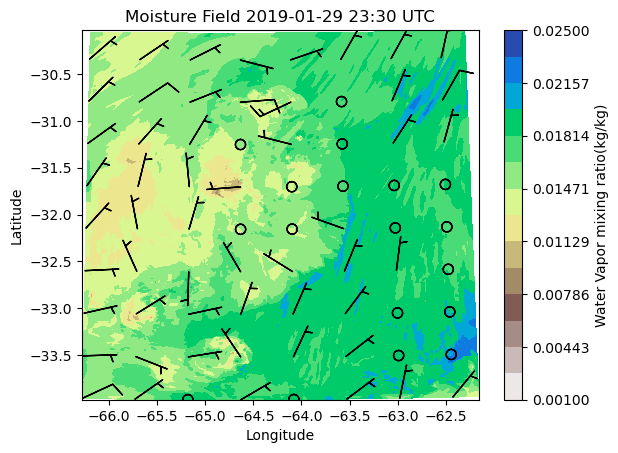
ds = xr.open_dataset(file_list[70])

theta = ds.QVAPOR[0,0,:,:]
u = ds.UMET10[0,:,:]
v = ds.VMET10[0,:,:]

space =100

cf=plt.contourf(ds.XLONG,ds.XLAT,theta, cmap='terrain_r', levels=np.linspace(0.001,0.025, 15))
plt.xlabel('Longitude')
plt.ylabel('Latitude')
time_label=plt.title('Moisture Field')
tx_time= plt.title(f"Moisture Field {pd.to_datetime(ds['Time'])[0]:%Y-%m-%d %H:%M} UTC")

ba = plt.barbs(ds.XLONG [::space, ::space], ds.XLAT[::space, ::space], u[::space, ::space],v[::space, ::space])
plt.colorbar(cf, label='Water Vapor mixing ratio(kg/kg)')

<matplotlib.colorbar.Colorbar at 0x7f8eae3d7710>

Cross Sections

path_staging = "/data/project/ARM_Summer_School_2024_Data/lasso_tutorial/cacti/lasso-cacti"
file_list = sorted(glob.glob(f'{path_staging}/20190129/eda09/base/les/subset_d3/corlasso_met_*'))

ntimes=73
ds= xr.open_mfdataset(file_list[:ntimes])

file_list = sorted(glob.glob(f'{path_staging}/20190129/eda09/base/les/subset_d3/corlasso_cld_*'))
ds2= xr.open_mfdataset(file_list[:ntimes])

# User settings...

# Case date and times to plot:
case_date = datetime(2019, 1, 29)
single_time = case_date + timedelta(hours=20, minutes=15)  # time for single-time plots

# Simulation selection within the case date:
ens_name = "eda09"
config_label = "base"
domain = 2



plot_lat= -32.1264  #S


# Next, we have to figure out which j-index to sample for the desired latitude. WRF's coordinate name for this dimension is south_north.
# We will ignore the map projection and pull along a single j index, which we will determine from the middle of the grid.
lats = ds2["XLAT"]
lons = ds2["XLONG"]
nlat, nlon = lons.shape
abslat = np.abs(lats.isel(west_east=int(nlon/2)) - plot_lat)
jloc = np.argmin(abslat.values)
lonslice = lons.isel(south_north=jloc)
hamsl_raw = ds['HAMSL'].isel(Time=0, south_north=jloc)  # height of each grid cell on the raw model levels


# ...and now the data we actually want to plot, which is clouds
plotdata_raw = 1000.*(
    ds2['QCLOUD'].sel(south_north=jloc) +
    ds2['QICE'].sel(south_north=jloc)
    )  # cloud water+ice mixing ratio converted go g/kg

#pcm=plotdata_raw.isel(Time=0).plot()



def plot_subsequent_frame(itime, plotdata_raw, pcm, tx_time, ba, ba_U, ba_V,ifreq):
    """
    Subroutine to plot the next frame of an animation after the first frame is already defined. 
    This is to be called by animation.FuncAnimation. 
    
    Note that some data is pulled from global scope. Variables accessed from outside the subroutine:
        pcm = pcolormesh object from the initial frame
        tx_time = text annotation object for the time label from the initial frame

        plotdata_raw = variable holding the time series of data to plot
        plot_lat = latitude being plotted (needed to reconstruct the title text)
    """
    print("plotting frame ", itime)

    # Overwrite the data in memory for the values displayed in the plot...
    # NOTE: This is technically a faux paux for WRF since the model levels are not constant in time. BE CAREFUL!
    #       However, in this situation the levels are not going to change so much as to make the plot visibly change much.
    pcm.set_array(plotdata_raw.isel(Time=itime).values.ravel())

    print(ba_U.isel(Time=itime).values[::ifreq, ::ifreq].shape)
    print(ba_V.isel(Time=itime).values[::ifreq, ::ifreq].shape) 
    

    #ba.set_UVC(ba_U.isel(Time=itime).values[::ifreq, ::ifreq].ravel(),ba_V.isel(Time=itime).values[::ifreq, ::ifreq].ravel())

    # Update the time label...
    time_label = f"{pd.to_datetime(plotdata_raw['Time'])[itime]:%Y-%m-%d %H:%M} UTC"
    tx_time.set_text(f"Cloud Condensate; \n{time_label}")




# end plot_subsequent_frame()

fig, ax = plt.subplots(1, 1, figsize=[8,3.5])
pcm= ax.pcolormesh(lonslice.values, hamsl_raw.values, plotdata_raw.isel(Time=0).values,
                   shading='auto',norm=Normalize(vmin=0,vmax=1.25))
#pcm=plotdata_raw.plot()
#theta = ds.QVAPOR[0,0,:,:]

da_u = ds["UMET"].isel(south_north=jloc)
da_v = ds["VMET"].isel(south_north=jloc)

space =100

cf=plt.contourf(ds.XLONG,ds.XLAT,theta)
#plt.xlabel('Longitude')
#plt.ylabel('Latitude')
tx_time= plt.title(f"Moisture Field {pd.to_datetime(plotdata_raw['Time'])[0]:%Y-%m-%d %H:%M} UTC")


lonslice2d = (lonslice+(hamsl_raw*0)).T
print(lonslice2d.T.shape)
#print(hamsl_raw.isel(Time=0).shape)
#print(da_u.isel(Time=0).shape)
da_u = ds["UMET"].isel(south_north=jloc)
da_v = ds["VMET"].isel(south_north=jloc)
ifreq = 10

print(lonslice2d.values[::ifreq,::ifreq].shape)
print(hamsl_raw.values[::ifreq,::ifreq].shape) 
print(da_u.isel(Time=0).values[::ifreq,::ifreq].shape)
print(da_v.isel(Time=0).values[::ifreq,::ifreq].shape)

#plt.barbs(lonslice2d.values[::ifreq,::ifreq], hamsl_raw.values[::ifreq,::ifreq], da_u.isel(Time=0).values[::ifreq,::ifreq], da_v.isel(Time=0).values[::ifreq,::ifreq],color='w')
# plt.pcolormesh(lonslice.values, hamsl_raw.isel(Time=0).values, da_v.isel(Time=0).values)
plt.show()


plt.colorbar(cf, label='Water Vapor mixing ratio(kg/kg)')



#-----------------------------------------------------------------------
# Now, update the underlying data in the plot for each subsequent frame...

# NOTE: See https://matplotlib.org/stable/api/_as_gen/matplotlib.animation.FuncAnimation.html for
#       explaination of how to use functools.partial for passing arguments to the redraw subroutine.
ani = animation.FuncAnimation(fig, 
                              partial(plot_subsequent_frame, plotdata_raw=plotdata_raw, pcm=pcm, tx_time=tx_time,ba=ba,ba_U=da_u,ba_V=da_v,ifreq=ifreq),
                              frames=range(ntimes))

# And save the results...
filename_mp4 = f"./corlasso_anim_qci_{case_date:%Y%m%d}00{ens_name}d{domain}_{config_label}.mp4"
fps = 6 if domain < 3 else 8  # set frame rate for dt=15 vs. 5 minutes
ani.save(filename_mp4, writer=animation.FFMpegWriter(fps=fps, bitrate=5000, codec="h264"), dpi=150)

/tmp/ipykernel_1683/1194218404.py:73: UserWarning: The input coordinates to pcolormesh are interpreted as cell centers, but are not monotonically increasing or decreasing. This may lead to incorrectly calculated cell edges, in which case, please supply explicit cell edges to pcolormesh.
  pcm= ax.pcolormesh(lonslice.values, hamsl_raw.values, plotdata_raw.isel(Time=0).values,

(750, 149)
(15, 75)
(15, 75)
(15, 75)
(15, 75)

plotting frame  0
(15, 75)
(15, 75)
plotting frame  0
(15, 75)
(15, 75)
plotting frame  1
(15, 75)
(15, 75)
plotting frame  2
(15, 75)
(15, 75)
plotting frame  3
(15, 75)
(15, 75)
plotting frame  4
(15, 75)
(15, 75)
plotting frame  5
(15, 75)
(15, 75)
plotting frame  6
(15, 75)
(15, 75)
plotting frame  7
(15, 75)
(15, 75)
plotting frame  8
(15, 75)
(15, 75)
plotting frame  9
(15, 75)
(15, 75)
plotting frame  10
(15, 75)
(15, 75)
plotting frame  11
(15, 75)
(15, 75)
plotting frame  12
(15, 75)
(15, 75)
plotting frame  13
(15, 75)
(15, 75)
plotting frame  14
(15, 75)
(15, 75)
plotting frame  15
(15, 75)
(15, 75)
plotting frame  16
(15, 75)
(15, 75)
plotting frame  17
(15, 75)
(15, 75)
plotting frame  18
(15, 75)
(15, 75)
plotting frame  19
(15, 75)
(15, 75)
plotting frame  20
(15, 75)
(15, 75)
plotting frame  21
(15, 75)
(15, 75)
plotting frame  22
(15, 75)
(15, 75)
plotting frame  23
(15, 75)
(15, 75)
plotting frame  24
(15, 75)
(15, 75)
plotting frame  25
(15, 75)
(15, 75)
plotting frame  26
(15, 75)
(15, 75)
plotting frame  27
(15, 75)
(15, 75)
plotting frame  28
(15, 75)
(15, 75)
plotting frame  29
(15, 75)
(15, 75)
plotting frame  30
(15, 75)
(15, 75)
plotting frame  31
(15, 75)
(15, 75)
plotting frame  32
(15, 75)
(15, 75)
plotting frame  33
(15, 75)
(15, 75)
plotting frame  34
(15, 75)
(15, 75)
plotting frame  35
(15, 75)
(15, 75)
plotting frame  36
(15, 75)
(15, 75)
plotting frame  37
(15, 75)
(15, 75)
plotting frame  38
(15, 75)
(15, 75)
plotting frame  39
(15, 75)
(15, 75)
plotting frame  40
(15, 75)
(15, 75)
plotting frame  41
(15, 75)
(15, 75)
plotting frame  42
(15, 75)
(15, 75)
plotting frame  43
(15, 75)
(15, 75)
plotting frame  44
(15, 75)
(15, 75)
plotting frame  45
(15, 75)
(15, 75)
plotting frame  46
(15, 75)
(15, 75)
plotting frame  47
(15, 75)
(15, 75)
plotting frame  48
(15, 75)
(15, 75)
plotting frame  49
(15, 75)
(15, 75)
plotting frame  50
(15, 75)
(15, 75)
plotting frame  51
(15, 75)
(15, 75)
plotting frame  52
(15, 75)
(15, 75)
plotting frame  53
(15, 75)
(15, 75)
plotting frame  54
(15, 75)
(15, 75)
plotting frame  55
(15, 75)
(15, 75)
plotting frame  56
(15, 75)
(15, 75)
plotting frame  57
(15, 75)
(15, 75)
plotting frame  58
(15, 75)
(15, 75)
plotting frame  59
(15, 75)
(15, 75)
plotting frame  60
(15, 75)
(15, 75)
plotting frame  61
(15, 75)
(15, 75)
plotting frame  62
(15, 75)
(15, 75)
plotting frame  63
(15, 75)
(15, 75)
plotting frame  64
(15, 75)
(15, 75)
plotting frame  65
(15, 75)
(15, 75)
plotting frame  66
(15, 75)
(15, 75)
plotting frame  67
(15, 75)
(15, 75)
plotting frame  68
(15, 75)
(15, 75)
plotting frame  69
(15, 75)
(15, 75)
plotting frame  70
(15, 75)
(15, 75)
plotting frame  71
(15, 75)
(15, 75)
plotting frame  72
(15, 75)
(15, 75)

<Figure size 640x480 with 0 Axes>

QCloud + QIce for Domain 2, 29-Jan-2019, EDA09 Forcing:

corlasso_anim_qci_2019012900eda09d2_base.mp4

ds

<xarray.Dataset> Size: 59GB
Dimensions:               (Time: 10, south_north: 865, west_east: 750,
                           bottom_top: 149)
Coordinates:
  * Time                  (Time) datetime64[ns] 80B 2019-01-29T06:00:00 ... 2...
    XLONG                 (south_north, west_east) float32 3MB dask.array<chunksize=(865, 750), meta=np.ndarray>
    XLAT                  (south_north, west_east) float32 3MB dask.array<chunksize=(865, 750), meta=np.ndarray>
    XTIME                 (Time) float32 40B dask.array<chunksize=(1,), meta=np.ndarray>
Dimensions without coordinates: south_north, west_east, bottom_top
Data variables: (12/52)
    ITIMESTEP             (Time) int32 40B dask.array<chunksize=(1,), meta=np.ndarray>
    MUTOT                 (Time, south_north, west_east) float32 26MB dask.array<chunksize=(1, 865, 750), meta=np.ndarray>
    HGT                   (Time, south_north, west_east) float32 26MB dask.array<chunksize=(1, 865, 750), meta=np.ndarray>
    HAMSL                 (Time, bottom_top, south_north, west_east) float32 4GB dask.array<chunksize=(1, 50, 289, 250), meta=np.ndarray>
    P_HYD                 (Time, bottom_top, south_north, west_east) float32 4GB dask.array<chunksize=(1, 50, 289, 250), meta=np.ndarray>
    PRESSURE              (Time, bottom_top, south_north, west_east) float32 4GB dask.array<chunksize=(1, 50, 289, 250), meta=np.ndarray>
    ...                    ...
    MULFC                 (Time, south_north, west_east) float32 26MB dask.array<chunksize=(1, 865, 750), meta=np.ndarray>
    MULNB                 (Time, south_north, west_east) float32 26MB dask.array<chunksize=(1, 865, 750), meta=np.ndarray>
    MULPL                 (Time, south_north, west_east) float32 26MB dask.array<chunksize=(1, 865, 750), meta=np.ndarray>
    MUCAPE                (Time, south_north, west_east) float32 26MB dask.array<chunksize=(1, 865, 750), meta=np.ndarray>
    MUCIN                 (Time, south_north, west_east) float32 26MB dask.array<chunksize=(1, 865, 750), meta=np.ndarray>
    REFL_10CM_MAX         (Time, south_north, west_east) float32 26MB dask.array<chunksize=(1, 865, 750), meta=np.ndarray>
Attributes: (12/39)
    DX:                          500.0
    DY:                          500.0
    SIMULATION_START_DATE:       2019-01-29_06:00:00
    WEST-EAST_GRID_DIMENSION:    751
    SOUTH-NORTH_GRID_DIMENSION:  866
    BOTTOM-TOP_GRID_DIMENSION:   150
    ...                          ...
    doi_isPartOf_lasso-cacti:    https://doi.org/10.5439/1905789
    doi_isDocumentedBy:          https://doi.org/10.2172/1905845
    doi_thisFileType:            https://doi.org/10.5439/1905819
    history:                     processed by user d3m088 on machine cirrus89...
    filename_user:               corlasso_met_2019012900eda09d3_base_M1.m1.20...
    filename_storage:            corlassomet2019012900eda09d3baseM1.m1.201901...

xarray.Dataset

• Dimensions:
  • Time: 10
  • south_north: 865
  • west_east: 750
  • bottom_top: 149
• Coordinates: (4)
  • Time
    (Time)
    datetime64[ns]
    2019-01-29T06:00:00 ... 2019-01-...

    array(['2019-01-29T06:00:00.000000000', '2019-01-29T06:15:00.000000000',
           '2019-01-29T06:30:00.000000000', '2019-01-29T06:45:00.000000000',
           '2019-01-29T07:00:00.000000000', '2019-01-29T07:15:00.000000000',
           '2019-01-29T07:30:00.000000000', '2019-01-29T07:45:00.000000000',
           '2019-01-29T08:00:00.000000000', '2019-01-29T08:15:00.000000000'],
          dtype='datetime64[ns]')

  • XLONG
    (south_north, west_east)
    float32
    dask.array<chunksize=(865, 750), meta=np.ndarray>

    Array Chunk Bytes 2.47 MiB 2.47 MiB Shape (865, 750) (865, 750) Dask graph 1 chunks in 45 graph layers Data type float32 numpy.ndarray

  • XLAT
    (south_north, west_east)
    float32
    dask.array<chunksize=(865, 750), meta=np.ndarray>

    Array Chunk Bytes 2.47 MiB 2.47 MiB Shape (865, 750) (865, 750) Dask graph 1 chunks in 45 graph layers Data type float32 numpy.ndarray

  • XTIME
    (Time)
    float32
    dask.array<chunksize=(1,), meta=np.ndarray>

    Array Chunk Bytes 40 B 4 B Shape (10,) (1,) Dask graph 10 chunks in 21 graph layers Data type float32 numpy.ndarray

• Data variables: (52)
  • ITIMESTEP
    (Time)
    int32
    dask.array<chunksize=(1,), meta=np.ndarray>

    description :

    WRF timestep number since run start

    units :

    Array Chunk Bytes 40 B 4 B Shape (10,) (1,) Dask graph 10 chunks in 21 graph layers Data type int32 numpy.ndarray

  • MUTOT
    (Time, south_north, west_east)
    float32
    dask.array<chunksize=(1, 865, 750), meta=np.ndarray>

    description :

    dry air mass in column

    units :

    Pa

    stagger :

    Array Chunk Bytes 24.75 MiB 2.47 MiB Shape (10, 865, 750) (1, 865, 750) Dask graph 10 chunks in 21 graph layers Data type float32 numpy.ndarray

  • HGT
    (Time, south_north, west_east)
    float32
    dask.array<chunksize=(1, 865, 750), meta=np.ndarray>

    description :

    Terrain Height

    units :

    m

    stagger :

    Array Chunk Bytes 24.75 MiB 2.47 MiB Shape (10, 865, 750) (1, 865, 750) Dask graph 10 chunks in 21 graph layers Data type float32 numpy.ndarray

  • HAMSL
    (Time, bottom_top, south_north, west_east)
    float32
    dask.array<chunksize=(1, 50, 289, 250), meta=np.ndarray>

    description :

    model height - [MSL] (mass grid)

    units :

    m

    stagger :

    Array Chunk Bytes 3.60 GiB 13.78 MiB Shape (10, 149, 865, 750) (1, 50, 289, 250) Dask graph 270 chunks in 21 graph layers Data type float32 numpy.ndarray

  • P_HYD
    (Time, bottom_top, south_north, west_east)
    float32
    dask.array<chunksize=(1, 50, 289, 250), meta=np.ndarray>

    description :

    hydrostatic pressure

    units :

    Pa

    stagger :

    Array Chunk Bytes 3.60 GiB 13.78 MiB Shape (10, 149, 865, 750) (1, 50, 289, 250) Dask graph 270 chunks in 21 graph layers Data type float32 numpy.ndarray

  • PRESSURE
    (Time, bottom_top, south_north, west_east)
    float32
    dask.array<chunksize=(1, 50, 289, 250), meta=np.ndarray>

    description :

    pressure

    units :

    hPa

    stagger :

    Array Chunk Bytes 3.60 GiB 13.78 MiB Shape (10, 149, 865, 750) (1, 50, 289, 250) Dask graph 270 chunks in 21 graph layers Data type float32 numpy.ndarray

  • ALT
    (Time, bottom_top, south_north, west_east)
    float32
    dask.array<chunksize=(1, 50, 289, 250), meta=np.ndarray>

    description :

    inverse density

    units :

    m3 kg-1

    stagger :

    Array Chunk Bytes 3.60 GiB 13.78 MiB Shape (10, 149, 865, 750) (1, 50, 289, 250) Dask graph 270 chunks in 21 graph layers Data type float32 numpy.ndarray

  • TEMPERATURE
    (Time, bottom_top, south_north, west_east)
    float32
    dask.array<chunksize=(1, 50, 289, 250), meta=np.ndarray>

    description :

    temperature

    units :

    K

    stagger :

    Array Chunk Bytes 3.60 GiB 13.78 MiB Shape (10, 149, 865, 750) (1, 50, 289, 250) Dask graph 270 chunks in 21 graph layers Data type float32 numpy.ndarray

  • THETA
    (Time, bottom_top, south_north, west_east)
    float32
    dask.array<chunksize=(1, 50, 289, 250), meta=np.ndarray>

    description :

    potential temperature

    units :

    K

    stagger :

    Array Chunk Bytes 3.60 GiB 13.78 MiB Shape (10, 149, 865, 750) (1, 50, 289, 250) Dask graph 270 chunks in 21 graph layers Data type float32 numpy.ndarray

  • THETA_E
    (Time, bottom_top, south_north, west_east)
    float32
    dask.array<chunksize=(1, 50, 289, 250), meta=np.ndarray>

    description :

    equivalent potential temperature

    units :

    K

    stagger :

    Array Chunk Bytes 3.60 GiB 13.78 MiB Shape (10, 149, 865, 750) (1, 50, 289, 250) Dask graph 270 chunks in 21 graph layers Data type float32 numpy.ndarray

  • QVAPOR
    (Time, bottom_top, south_north, west_east)
    float32
    dask.array<chunksize=(1, 50, 289, 250), meta=np.ndarray>

    description :

    Water vapor mixing ratio

    units :

    kg kg-1

    stagger :

    Array Chunk Bytes 3.60 GiB 13.78 MiB Shape (10, 149, 865, 750) (1, 50, 289, 250) Dask graph 270 chunks in 21 graph layers Data type float32 numpy.ndarray

  • RH
    (Time, bottom_top, south_north, west_east)
    float32
    dask.array<chunksize=(1, 50, 289, 250), meta=np.ndarray>

    description :

    relative humidity

    units :

    %

    stagger :

    Array Chunk Bytes 3.60 GiB 13.78 MiB Shape (10, 149, 865, 750) (1, 50, 289, 250) Dask graph 270 chunks in 21 graph layers Data type float32 numpy.ndarray

  • UA
    (Time, bottom_top, south_north, west_east)
    float32
    dask.array<chunksize=(1, 50, 289, 250), meta=np.ndarray>

    description :

    destaggered u-wind component

    units :

    m s-1

    stagger :

    Array Chunk Bytes 3.60 GiB 13.78 MiB Shape (10, 149, 865, 750) (1, 50, 289, 250) Dask graph 270 chunks in 21 graph layers Data type float32 numpy.ndarray

  • VA
    (Time, bottom_top, south_north, west_east)
    float32
    dask.array<chunksize=(1, 50, 289, 250), meta=np.ndarray>

    description :

    destaggered v-wind component

    units :

    m s-1

    stagger :

    Array Chunk Bytes 3.60 GiB 13.78 MiB Shape (10, 149, 865, 750) (1, 50, 289, 250) Dask graph 270 chunks in 21 graph layers Data type float32 numpy.ndarray

  • WA
    (Time, bottom_top, south_north, west_east)
    float32
    dask.array<chunksize=(1, 50, 289, 250), meta=np.ndarray>

    description :

    destaggered w-wind component

    units :

    m s-1

    stagger :

    Array Chunk Bytes 3.60 GiB 13.78 MiB Shape (10, 149, 865, 750) (1, 50, 289, 250) Dask graph 270 chunks in 21 graph layers Data type float32 numpy.ndarray

  • UMET
    (Time, bottom_top, south_north, west_east)
    float32
    dask.array<chunksize=(1, 50, 289, 250), meta=np.ndarray>

    description :

    earth-relative u-wind component

    units :

    m s-1

    stagger :

    Array Chunk Bytes 3.60 GiB 13.78 MiB Shape (10, 149, 865, 750) (1, 50, 289, 250) Dask graph 270 chunks in 21 graph layers Data type float32 numpy.ndarray

  • VMET
    (Time, bottom_top, south_north, west_east)
    float32
    dask.array<chunksize=(1, 50, 289, 250), meta=np.ndarray>

    description :

    earth-relative v-wind component

    units :

    m s-1

    stagger :

    Array Chunk Bytes 3.60 GiB 13.78 MiB Shape (10, 149, 865, 750) (1, 50, 289, 250) Dask graph 270 chunks in 21 graph layers Data type float32 numpy.ndarray

  • POTVORT
    (Time, bottom_top, south_north, west_east)
    float32
    dask.array<chunksize=(1, 50, 289, 250), meta=np.ndarray>

    description :

    potential vorticity

    units :

    PVU

    stagger :

    Array Chunk Bytes 3.60 GiB 13.78 MiB Shape (10, 149, 865, 750) (1, 50, 289, 250) Dask graph 270 chunks in 21 graph layers Data type float32 numpy.ndarray

  • PSFC
    (Time, south_north, west_east)
    float32
    dask.array<chunksize=(1, 865, 750), meta=np.ndarray>

    description :

    SFC PRESSURE

    units :

    Pa

    stagger :

    Array Chunk Bytes 24.75 MiB 2.47 MiB Shape (10, 865, 750) (1, 865, 750) Dask graph 10 chunks in 21 graph layers Data type float32 numpy.ndarray

  • SLP
    (Time, south_north, west_east)
    float32
    dask.array<chunksize=(1, 865, 750), meta=np.ndarray>

    description :

    sea level pressure

    units :

    hPa

    stagger :

    Array Chunk Bytes 24.75 MiB 2.47 MiB Shape (10, 865, 750) (1, 865, 750) Dask graph 10 chunks in 21 graph layers Data type float32 numpy.ndarray

  • Q2
    (Time, south_north, west_east)
    float32
    dask.array<chunksize=(1, 865, 750), meta=np.ndarray>

    description :

    QV at 2 M

    units :

    kg kg-1

    stagger :

    Array Chunk Bytes 24.75 MiB 2.47 MiB Shape (10, 865, 750) (1, 865, 750) Dask graph 10 chunks in 21 graph layers Data type float32 numpy.ndarray

  • T2
    (Time, south_north, west_east)
    float32
    dask.array<chunksize=(1, 865, 750), meta=np.ndarray>

    description :

    TEMP at 2 M

    units :

    K

    stagger :

    Array Chunk Bytes 24.75 MiB 2.47 MiB Shape (10, 865, 750) (1, 865, 750) Dask graph 10 chunks in 21 graph layers Data type float32 numpy.ndarray

  • TH2
    (Time, south_north, west_east)
    float32
    dask.array<chunksize=(1, 865, 750), meta=np.ndarray>

    description :

    POT TEMP at 2 M

    units :

    K

    stagger :

    Array Chunk Bytes 24.75 MiB 2.47 MiB Shape (10, 865, 750) (1, 865, 750) Dask graph 10 chunks in 21 graph layers Data type float32 numpy.ndarray

  • U10
    (Time, south_north, west_east)
    float32
    dask.array<chunksize=(1, 865, 750), meta=np.ndarray>

    description :

    U at 10 M

    units :

    m s-1

    stagger :

    Array Chunk Bytes 24.75 MiB 2.47 MiB Shape (10, 865, 750) (1, 865, 750) Dask graph 10 chunks in 21 graph layers Data type float32 numpy.ndarray

  • V10
    (Time, south_north, west_east)
    float32
    dask.array<chunksize=(1, 865, 750), meta=np.ndarray>

    description :

    V at 10 M

    units :

    m s-1

    stagger :

    Array Chunk Bytes 24.75 MiB 2.47 MiB Shape (10, 865, 750) (1, 865, 750) Dask graph 10 chunks in 21 graph layers Data type float32 numpy.ndarray

  • UMET10
    (Time, south_north, west_east)
    float32
    dask.array<chunksize=(1, 865, 750), meta=np.ndarray>

    description :

    earth-relative 10-m u-wind component

    units :

    m s-1

    stagger :

    Array Chunk Bytes 24.75 MiB 2.47 MiB Shape (10, 865, 750) (1, 865, 750) Dask graph 10 chunks in 21 graph layers Data type float32 numpy.ndarray

  • VMET10
    (Time, south_north, west_east)
    float32
    dask.array<chunksize=(1, 865, 750), meta=np.ndarray>

    description :

    earth-relative 10-m v-wind component

    units :

    m s-1

    stagger :

    Array Chunk Bytes 24.75 MiB 2.47 MiB Shape (10, 865, 750) (1, 865, 750) Dask graph 10 chunks in 21 graph layers Data type float32 numpy.ndarray

  • SHEAR_MAG_SFC-TO-1KM
    (Time, south_north, west_east)
    float32
    dask.array<chunksize=(1, 865, 750), meta=np.ndarray>

    units :

    m s-1

    stagger :

    description :

    bulk wind-shear magnitude, sfc to 1000.0

    Array Chunk Bytes 24.75 MiB 2.47 MiB Shape (10, 865, 750) (1, 865, 750) Dask graph 10 chunks in 21 graph layers Data type float32 numpy.ndarray

  • SHEAR_DIR_SFC-TO-1KM
    (Time, south_north, west_east)
    float32
    dask.array<chunksize=(1, 865, 750), meta=np.ndarray>

    units :

    degrees

    stagger :

    description :

    bulk wind-shear direction, sfc to 1000.0

    Array Chunk Bytes 24.75 MiB 2.47 MiB Shape (10, 865, 750) (1, 865, 750) Dask graph 10 chunks in 21 graph layers Data type float32 numpy.ndarray

  • SHEAR_MAG_SFC-TO-3KM
    (Time, south_north, west_east)
    float32
    dask.array<chunksize=(1, 865, 750), meta=np.ndarray>

    units :

    m s-1

    stagger :

    description :

    bulk wind-shear magnitude, sfc to 3000.0

    Array Chunk Bytes 24.75 MiB 2.47 MiB Shape (10, 865, 750) (1, 865, 750) Dask graph 10 chunks in 21 graph layers Data type float32 numpy.ndarray

  • SHEAR_DIR_SFC-TO-3KM
    (Time, south_north, west_east)
    float32
    dask.array<chunksize=(1, 865, 750), meta=np.ndarray>

    units :

    degrees

    stagger :

    description :

    bulk wind-shear direction, sfc to 3000.0

    Array Chunk Bytes 24.75 MiB 2.47 MiB Shape (10, 865, 750) (1, 865, 750) Dask graph 10 chunks in 21 graph layers Data type float32 numpy.ndarray

  • SHEAR_MAG_SFC-TO-6KM
    (Time, south_north, west_east)
    float32
    dask.array<chunksize=(1, 865, 750), meta=np.ndarray>

    units :

    m s-1

    stagger :

    description :

    bulk wind-shear magnitude, sfc to 6000.0

    Array Chunk Bytes 24.75 MiB 2.47 MiB Shape (10, 865, 750) (1, 865, 750) Dask graph 10 chunks in 21 graph layers Data type float32 numpy.ndarray

  • SHEAR_DIR_SFC-TO-6KM
    (Time, south_north, west_east)
    float32
    dask.array<chunksize=(1, 865, 750), meta=np.ndarray>

    units :

    degrees

    stagger :

    description :

    bulk wind-shear direction, sfc to 6000.0

    Array Chunk Bytes 24.75 MiB 2.47 MiB Shape (10, 865, 750) (1, 865, 750) Dask graph 10 chunks in 21 graph layers Data type float32 numpy.ndarray

  • SHEAR_MAG_SFC-TO-9KM
    (Time, south_north, west_east)
    float32
    dask.array<chunksize=(1, 865, 750), meta=np.ndarray>

    units :

    m s-1

    stagger :

    description :

    bulk wind-shear magnitude, sfc to 9000.0

    Array Chunk Bytes 24.75 MiB 2.47 MiB Shape (10, 865, 750) (1, 865, 750) Dask graph 10 chunks in 21 graph layers Data type float32 numpy.ndarray

  • SHEAR_DIR_SFC-TO-9KM
    (Time, south_north, west_east)
    float32
    dask.array<chunksize=(1, 865, 750), meta=np.ndarray>

    units :

    degrees

    stagger :

    description :

    bulk wind-shear direction, sfc to 9000.0

    Array Chunk Bytes 24.75 MiB 2.47 MiB Shape (10, 865, 750) (1, 865, 750) Dask graph 10 chunks in 21 graph layers Data type float32 numpy.ndarray

  • RAINNC
    (Time, south_north, west_east)
    float32
    dask.array<chunksize=(1, 865, 750), meta=np.ndarray>

    description :

    ACCUMULATED TOTAL GRID SCALE PRECIPITATION

    units :

    mm

    stagger :

    Array Chunk Bytes 24.75 MiB 2.47 MiB Shape (10, 865, 750) (1, 865, 750) Dask graph 10 chunks in 21 graph layers Data type float32 numpy.ndarray

  • SNOWNC
    (Time, south_north, west_east)
    float32
    dask.array<chunksize=(1, 865, 750), meta=np.ndarray>

    description :

    ACCUMULATED TOTAL GRID SCALE SNOW AND ICE

    units :

    mm

    stagger :

    Array Chunk Bytes 24.75 MiB 2.47 MiB Shape (10, 865, 750) (1, 865, 750) Dask graph 10 chunks in 21 graph layers Data type float32 numpy.ndarray

  • GRAUPELNC
    (Time, south_north, west_east)
    float32
    dask.array<chunksize=(1, 865, 750), meta=np.ndarray>

    description :

    ACCUMULATED TOTAL GRID SCALE GRAUPEL

    units :

    mm

    stagger :

    Array Chunk Bytes 24.75 MiB 2.47 MiB Shape (10, 865, 750) (1, 865, 750) Dask graph 10 chunks in 21 graph layers Data type float32 numpy.ndarray

  • SR
    (Time, south_north, west_east)
    float32
    dask.array<chunksize=(1, 865, 750), meta=np.ndarray>

    description :

    fraction of frozen precipitation

    units :

    -

    stagger :

    Array Chunk Bytes 24.75 MiB 2.47 MiB Shape (10, 865, 750) (1, 865, 750) Dask graph 10 chunks in 21 graph layers Data type float32 numpy.ndarray

  • MLLCL
    (Time, south_north, west_east)
    float32
    dask.array<chunksize=(1, 865, 750), meta=np.ndarray>

    description :

    most-unstable lifting condensation level

    units :

    m

    stagger :

    Array Chunk Bytes 24.75 MiB 2.47 MiB Shape (10, 865, 750) (1, 865, 750) Dask graph 10 chunks in 21 graph layers Data type float32 numpy.ndarray

  • MLLFC
    (Time, south_north, west_east)
    float32
    dask.array<chunksize=(1, 865, 750), meta=np.ndarray>

    description :

    most-unstable level of free convection

    units :

    m

    stagger :

    Array Chunk Bytes 24.75 MiB 2.47 MiB Shape (10, 865, 750) (1, 865, 750) Dask graph 10 chunks in 21 graph layers Data type float32 numpy.ndarray

  • MLLNB
    (Time, south_north, west_east)
    float32
    dask.array<chunksize=(1, 865, 750), meta=np.ndarray>

    description :

    most-unstable level of neutral buoyancy

    units :

    m

    stagger :

    Array Chunk Bytes 24.75 MiB 2.47 MiB Shape (10, 865, 750) (1, 865, 750) Dask graph 10 chunks in 21 graph layers Data type float32 numpy.ndarray

  • MLLPL
    (Time, south_north, west_east)
    float32
    dask.array<chunksize=(1, 865, 750), meta=np.ndarray>

    description :

    most-unstable lifted parcel level

    units :

    m

    stagger :

    Array Chunk Bytes 24.75 MiB 2.47 MiB Shape (10, 865, 750) (1, 865, 750) Dask graph 10 chunks in 21 graph layers Data type float32 numpy.ndarray

  • MLCAPE
    (Time, south_north, west_east)
    float32
    dask.array<chunksize=(1, 865, 750), meta=np.ndarray>

    description :

    most-unstable convective available potential energy

    units :

    J kg-1

    stagger :

    Array Chunk Bytes 24.75 MiB 2.47 MiB Shape (10, 865, 750) (1, 865, 750) Dask graph 10 chunks in 21 graph layers Data type float32 numpy.ndarray

  • MLCIN
    (Time, south_north, west_east)
    float32
    dask.array<chunksize=(1, 865, 750), meta=np.ndarray>

    description :

    most-unstable convective inhibition

    units :

    J kg-1

    stagger :

    Array Chunk Bytes 24.75 MiB 2.47 MiB Shape (10, 865, 750) (1, 865, 750) Dask graph 10 chunks in 21 graph layers Data type float32 numpy.ndarray

  • MULCL
    (Time, south_north, west_east)
    float32
    dask.array<chunksize=(1, 865, 750), meta=np.ndarray>

    description :

    most-unstable lifting condensation level

    units :

    m

    stagger :

    Array Chunk Bytes 24.75 MiB 2.47 MiB Shape (10, 865, 750) (1, 865, 750) Dask graph 10 chunks in 21 graph layers Data type float32 numpy.ndarray

  • MULFC
    (Time, south_north, west_east)
    float32
    dask.array<chunksize=(1, 865, 750), meta=np.ndarray>

    description :

    most-unstable level of free convection

    units :

    m

    stagger :

    Array Chunk Bytes 24.75 MiB 2.47 MiB Shape (10, 865, 750) (1, 865, 750) Dask graph 10 chunks in 21 graph layers Data type float32 numpy.ndarray

  • MULNB
    (Time, south_north, west_east)
    float32
    dask.array<chunksize=(1, 865, 750), meta=np.ndarray>

    description :

    most-unstable level of neutral buoyancy

    units :

    m

    stagger :

    Array Chunk Bytes 24.75 MiB 2.47 MiB Shape (10, 865, 750) (1, 865, 750) Dask graph 10 chunks in 21 graph layers Data type float32 numpy.ndarray

  • MULPL
    (Time, south_north, west_east)
    float32
    dask.array<chunksize=(1, 865, 750), meta=np.ndarray>

    description :

    most-unstable lifted parcel level

    units :

    m

    stagger :

    Array Chunk Bytes 24.75 MiB 2.47 MiB Shape (10, 865, 750) (1, 865, 750) Dask graph 10 chunks in 21 graph layers Data type float32 numpy.ndarray

  • MUCAPE
    (Time, south_north, west_east)
    float32
    dask.array<chunksize=(1, 865, 750), meta=np.ndarray>

    description :

    most-unstable convective available potential energy

    units :

    J kg-1

    stagger :

    Array Chunk Bytes 24.75 MiB 2.47 MiB Shape (10, 865, 750) (1, 865, 750) Dask graph 10 chunks in 21 graph layers Data type float32 numpy.ndarray

  • MUCIN
    (Time, south_north, west_east)
    float32
    dask.array<chunksize=(1, 865, 750), meta=np.ndarray>

    description :

    most-unstable convective inhibition

    units :

    J kg-1

    stagger :

    Array Chunk Bytes 24.75 MiB 2.47 MiB Shape (10, 865, 750) (1, 865, 750) Dask graph 10 chunks in 21 graph layers Data type float32 numpy.ndarray

  • REFL_10CM_MAX
    (Time, south_north, west_east)
    float32
    dask.array<chunksize=(1, 865, 750), meta=np.ndarray>

    description :

    column-maximum radar reflectivity (lambda = 10 cm)

    units :

    dBZ

    stagger :

    Array Chunk Bytes 24.75 MiB 2.47 MiB Shape (10, 865, 750) (1, 865, 750) Dask graph 10 chunks in 21 graph layers Data type float32 numpy.ndarray

• Indexes: (1)
  • Time
    PandasIndex

    PandasIndex(DatetimeIndex(['2019-01-29 06:00:00', '2019-01-29 06:15:00',
                   '2019-01-29 06:30:00', '2019-01-29 06:45:00',
                   '2019-01-29 07:00:00', '2019-01-29 07:15:00',
                   '2019-01-29 07:30:00', '2019-01-29 07:45:00',
                   '2019-01-29 08:00:00', '2019-01-29 08:15:00'],
                  dtype='datetime64[ns]', name='Time', freq=None))

• Attributes: (39)

  DX :

  500.0

  DY :

  500.0

  SIMULATION_START_DATE :

  2019-01-29_06:00:00

  WEST-EAST_GRID_DIMENSION :

  751

  SOUTH-NORTH_GRID_DIMENSION :

  866

  BOTTOM-TOP_GRID_DIMENSION :

  150

  GRIDTYPE :

  C

  CEN_LAT :

  -32.01111

  CEN_LON :

  -64.23425

  TRUELAT1 :

  -30.0

  TRUELAT2 :

  -60.0

  MOAD_CEN_LAT :

  -32.500015

  STAND_LON :

  -64.728

  POLE_LAT :

  90.0

  POLE_LON :

  0.0

  MAP_PROJ :

  1

  MAP_PROJ_CHAR :

  Lambert Conformal

  run_name :

  eda09_2019012900_base

  model_type :

  WRF

  model_version :

  NCAR V4.3.1 + LASSO modifications

  model_source_repository :

  https://code.arm.gov/lasso/lasso-cacti/lasso-wrf-cacti/

  model_source_git_hash :

  3e761eac

  subset_source_repository :

  https://code.arm.gov/lasso/lasso-cacti/subsetwrf

  subset_source_git_hash :

  99902f2

  domain_num :

  3

  input_source :

  /gpfs/wolf/cli120/world-shared/d3m088/cacti/staged_runs/20190129/eda09/base/les/out_d3

  site_id :

  cor

  platform_id :

  corlasso

  facility_designation :

  M1

  location_description :

  Cloud, Aerosol, and Complex Terrain Interactions (CACTI), Cordoba, Argentina

  data_level :

  m1

  datastream :

  corlasso_sub_met

  contact :

  lasso@arm.gov, LASSO PI: William Gustafson (PNNL, william.gustafson@pnnl.gov), LASSO Co-PI: Andrew Vogelmann (BNL)

  doi_isPartOf_lasso-cacti :

  https://doi.org/10.5439/1905789

  doi_isDocumentedBy :

  https://doi.org/10.2172/1905845

  doi_thisFileType :

  https://doi.org/10.5439/1905819

  history :

  processed by user d3m088 on machine cirrus89.ccs.ornl.gov at 23-Jan-2023 06:50 using subsetwrf.py

  filename_user :

  corlasso_met_2019012900eda09d3_base_M1.m1.20190129.060000.nc

  filename_storage :

  corlassomet2019012900eda09d3baseM1.m1.20190129.060000.nc

print(ds)

<xarray.Dataset> Size: 39GB
Dimensions:      (Time: 10, bottom_top: 149, south_north: 865, west_east: 750)
Coordinates:
  * Time         (Time) datetime64[ns] 80B 2019-01-29T06:00:00 ... 2019-01-29...
    XLONG        (south_north, west_east) float32 3MB dask.array<chunksize=(865, 750), meta=np.ndarray>
    XLAT         (south_north, west_east) float32 3MB dask.array<chunksize=(865, 750), meta=np.ndarray>
    XTIME        (Time) float32 40B dask.array<chunksize=(1,), meta=np.ndarray>
Dimensions without coordinates: bottom_top, south_north, west_east
Data variables: (12/14)
    ITIMESTEP    (Time) int32 40B dask.array<chunksize=(1,), meta=np.ndarray>
    QCLOUD       (Time, bottom_top, south_north, west_east) float32 4GB dask.array<chunksize=(1, 50, 289, 250), meta=np.ndarray>
    QRAIN        (Time, bottom_top, south_north, west_east) float32 4GB dask.array<chunksize=(1, 50, 289, 250), meta=np.ndarray>
    QICE         (Time, bottom_top, south_north, west_east) float32 4GB dask.array<chunksize=(1, 50, 289, 250), meta=np.ndarray>
    QSNOW        (Time, bottom_top, south_north, west_east) float32 4GB dask.array<chunksize=(1, 50, 289, 250), meta=np.ndarray>
    QGRAUP       (Time, bottom_top, south_north, west_east) float32 4GB dask.array<chunksize=(1, 50, 289, 250), meta=np.ndarray>
    ...           ...
    REFL_10CM    (Time, bottom_top, south_north, west_east) float32 4GB dask.array<chunksize=(1, 50, 289, 250), meta=np.ndarray>
    CLDFRA       (Time, bottom_top, south_north, west_east) float32 4GB dask.array<chunksize=(1, 50, 289, 250), meta=np.ndarray>
    LWP          (Time, south_north, west_east) float32 26MB dask.array<chunksize=(1, 865, 750), meta=np.ndarray>
    IWP          (Time, south_north, west_east) float32 26MB dask.array<chunksize=(1, 865, 750), meta=np.ndarray>
    PRECIPWATER  (Time, south_north, west_east) float32 26MB dask.array<chunksize=(1, 865, 750), meta=np.ndarray>
    QNCLOUD      (Time, bottom_top, south_north, west_east) float32 4GB dask.array<chunksize=(1, 50, 289, 250), meta=np.ndarray>
Attributes: (12/39)
    DX:                          500.0
    DY:                          500.0
    SIMULATION_START_DATE:       2019-01-29_06:00:00
    WEST-EAST_GRID_DIMENSION:    751
    SOUTH-NORTH_GRID_DIMENSION:  866
    BOTTOM-TOP_GRID_DIMENSION:   150
    ...                          ...
    doi_isPartOf_lasso-cacti:    https://doi.org/10.5439/1905789
    doi_isDocumentedBy:          https://doi.org/10.2172/1905845
    doi_thisFileType:            https://doi.org/10.5439/1905813
    history:                     processed by user d3m088 on machine cirrus74...
    filename_user:               corlasso_cld_2019012900eda09d3_base_M1.m1.20...
    filename_storage:            corlassocld2019012900eda09d3baseM1.m1.201901...

print(theta.shape)
print(ds.THETA_E.shape)
print(ds2.QCLOUD.shape)

(865, 750)
(10, 149, 865, 750)
(10, 149, 865, 750)

print(lonslice.values.shape)
print(hamsl_raw.values.shape)
print(da_u.values.shape) 
print(da_v.values.shape)

(750,)
(149, 750)
(10, 149, 750)
(10, 149, 750)