Convection initiation in Sierras de Cordoba

Overview

We will look at the 2019-01-29 convective storm near the Sierras de Cordoba

Prerequisites

Concepts	Importance	Notes
Intro to Cartopy	Necessary
Understanding of NetCDF	Helpful	Familiarity with metadata structure

Time to learn: 10 minutes

Imports

Let’s import our required libraries

import act
import xarray as xr
import cmweather
import matplotlib.pyplot as plt
import numpy as np
import pyart
import hvplot.xarray
import holoviews as hv
import glob
import xradar as xd
import cartopy.crs as ccrs
from dask.distributed import Client, LocalCluster
from functools import partial
hv.extension("bokeh")

## You are using the Python ARM Radar Toolkit (Py-ART), an open source
## library for working with weather radar data. Py-ART is partly
## supported by the U.S. Department of Energy as part of the Atmospheric
## Radiation Measurement (ARM) Climate Research Facility, an Office of
## Science user facility.
##
## If you use this software to prepare a publication, please cite:
##
##     JJ Helmus and SM Collis, JORS 2016, doi: 10.5334/jors.119

Dask Cluster

Let’s spin up our local cluster using Dask

client = Client(LocalCluster())

CACTI Domain Overview

CSAPR_lat = float(radar.latitude.values)
CSAPR_lon = float(radar.longitude.values)

cf = plt.contourf(ds.XLONG, ds.XLAT, ds.HGT[0,:,:], cmap='terrain', levels=np.arange(0, 2500, 50))
plt.scatter(CSAPR_lon, CSAPR_lat, s=50, c='tab:red', label='ARM Site')
plt.title('CACTI Domain', fontsize=15)
plt.colorbar(cf, label='Height (m)')
plt.legend()

<matplotlib.legend.Legend at 0x7fa060a4c2d0>

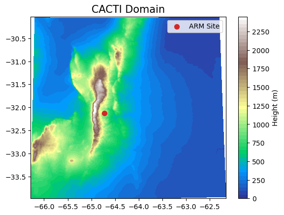
../_images/25a168596fffda04cdf1050a9e426c69326970914a8b6c00b9977c51da86b1c3.png

Now let’s examine the convection occurring during this particular day. To do this, we’ll use one of the radar files we imported above.

vel_plot = radar['sweep_0']["mean_doppler_velocity"].hvplot.quadmesh(x="x", y="y", cmap="balance", 
                                                          height=300, width=400, 
                                                          clim=(-20, 20),
                                                          rasterize=True)

ref_plot = radar['sweep_0']["reflectivity"].hvplot.quadmesh(x="x", y="y", cmap="ChaseSpectral", 
                                                          height=300, width=400, 
                                                          clim=(-20, 70),
                                                          rasterize=True)

ref_plot+vel_plot

We can see that all of the storms seem to be forming along one particular area. It looks like this might be the mountain range in the center of the CACTI domain shown above, but let’s overlay terrain on the radar image to verify this.

proj_crs = xd.georeference.get_crs(radar["sweep_0"].ds)
cart_crs = ccrs.Projection(proj_crs)

fig = plt.figure(figsize=(9, 9))
ax = fig.add_subplot(111, projection=ccrs.PlateCarree())
radar["sweep_0"]["reflectivity"].plot(
    x="x",
    y="y",
    cmap="ChaseSpectral",
    transform=cart_crs,
    cbar_kwargs=dict(pad=0.075, shrink=0.75),
    vmin=-20,
    vmax=70
)
ax.coastlines()
ax.gridlines(draw_labels=True)

ax.set_xlim([-66,-63.5])
ax.set_ylim([-33.2, -31])

cf = plt.contour(ds.XLONG, ds.XLAT, ds.HGT[0,:,:], cmap='terrain', levels=np.arange(0, 2500, 350), 
                 transform=ccrs.PlateCarree())

/data/project/jupyterhub/notebook-envs/arm-summer-school-2024-env/lib/python3.11/site-packages/cartopy/mpl/geoaxes.py:1768: UserWarning: The input coordinates to pcolormesh are interpreted as cell centers, but are not monotonically increasing or decreasing. This may lead to incorrectly calculated cell edges, in which case, please supply explicit cell edges to pcolormesh.
  result = super().pcolormesh(*args, **kwargs)

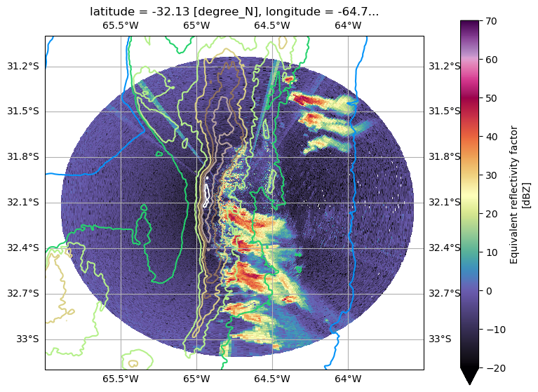
../_images/2bd99d3704bed93ff27eef8b95005a272a5ae296eb35daff313014125d78f54e.png

As we suspected, the storms are all located just east of the Sierras de Cordoba. This leads us to our hypothesis…

Science Question

How is deep convection initiation controlled by local and regional meteorological conditions (Thunderstorm life cycle)as well as geography?

Project Scope

Learning how to use LASSO simulation and ARM data.
Understand how convection is initiated in our domain by looking at measurements
Where convection is initiated in our domain of study
Comparison between observation and simulations

Hypothesis

Convection initiation near the ARM site is caused largely by orographic effects, surface heating, and advection of moisture from the Pacific.

Radar reflectivity plots

CSARP

We found in total 15 files for the 2021-01-29 deep convective storms as follows

files = sorted(glob.glob('corcsapr2cmacppiM1.c1/*'))
files[:3]

['corcsapr2cmacppiM1.c1/corcsapr2cmacppiM1.c1.20190129.130003.nc',
 'corcsapr2cmacppiM1.c1/corcsapr2cmacppiM1.c1.20190129.131503.nc',
 'corcsapr2cmacppiM1.c1/corcsapr2cmacppiM1.c1.20190129.133003.nc']

Summary

Add one final --- marking the end of your body of content, and then conclude with a brief single paragraph summarizing at a high level the key pieces that were learned and how they tied to your objectives. Look to reiterate what the most important takeaways were.

What’s next?

Let Jupyter book tie this to the next (sequential) piece of content that people could move on to down below and in the sidebar. However, if this page uniquely enables your reader to tackle other nonsequential concepts throughout this book, or even external content, link to it here!

Resources and references

Finally, be rigorous in your citations and references as necessary. Give credit where credit is due. Also, feel free to link to relevant external material, further reading, documentation, etc. Then you’re done! Give yourself a quick review, a high five, and send us a pull request. A few final notes:

Kernel > Restart Kernel and Run All Cells... to confirm that your notebook will cleanly run from start to finish
Kernel > Restart Kernel and Clear All Outputs... before committing your notebook, our machines will do the heavy lifting
Take credit! Provide author contact information if you’d like; if so, consider adding information here at the bottom of your notebook
Give credit! Attribute appropriate authorship for referenced code, information, images, etc.
Only include what you’re legally allowed: no copyright infringement or plagiarism

Thank you for your contribution!